This article explains how to optimize performance for an Amazon Redshift data warehouse that uses a star schema design. Many of these techniques will also work with other schema designs. We’ll talk about considerations for migrating data, when to use distribution styles and sort keys, various ways to optimize Amazon Redshift performance with star schemas, and how to identify and fix performance bottlenecks.

Amazon Redshift is a fully managed, petabyte-scale data warehouse service in the cloud. Amazon Redshift offers you fast query performance when analyzing virtually any size dataset using the same business intelligence applications you use today. Amazon Redshift uses many techniques to achieve fast query performance at scale, including multi-node parallel operations, hardware optimization, network optimization, and data compression. At the same time, Amazon Redshift minimizes operational overhead by freeing you from the hassle associated with provisioning, patching, backing up, restoring, monitoring, securing, and scaling a data warehouse cluster. For a detailed architecture overview of the Amazon Redshift service and optimization techniques, see the Amazon Redshift system overview.

To get in depth knowledge on AWS you can enroll for free live demo AWS Online Course

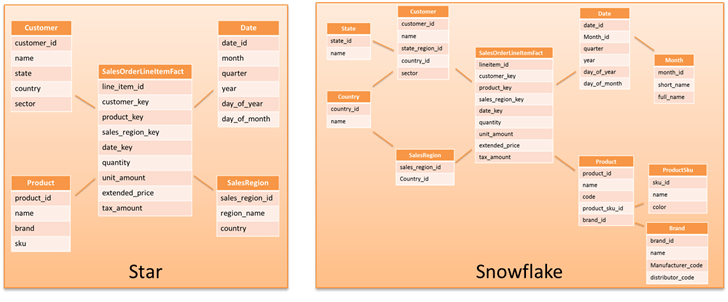
Many business intelligence solutions use a star schema or a normalized variation called a snowflake schema. Such solutions typically have tooling that depends upon a star schema design. Star schemas are organized around a central fact table that contains measurements for a specific event, such as a sold item. The fact table has foreign key relationships to one or more dimension tables that contain descriptive attribute information for the sold item, such as customer or product. Snowflake schemas extend the concept by further normalizing the dimensions into multiple tables. For example, a product dimension may have the brand in a separate table. For more information, see star schema and snowflake schema.

The Amazon Redshift design accommodates all types of data models, including 3NF, denormalized tables, and star and snowflake schemas. You should start from the assumption that your existing data model design will just work on Amazon Redshift. Most customers experience significantly better performance when migrating their existing data models to Amazon Redshift largely unchanged, though you should test for performance using either the actual or a representative dataset to ensure that your data model design and query patterns perform well before putting the workload into production.

Optimizations for Star Schemas

Amazon Redshift automatically detects star schema data structures and has built-in optimizations for efficiently querying this data. You also have a number of optimization options under your control that affect query performance whether you are using a star schema or another data model. The following sections explain how to apply these optimizations in the context of a star schema.

Primary and Foreign Key Constraints

When you move your data model to Amazon Redshift, you can declare your primary and foreign key relationships. Even though Amazon Redshift does not currently enforce these relationships, the query optimizer uses them as a hint when it analyzes a query. In certain circumstances, Amazon Redshift uses this information to optimize the query by eliminating redundant joins. Generally, the query optimizer detects redundant joins without constraints defined if you keep statistics up to date by running the ANALYZE command as described later in this article.

Learn for more AWS Interview Questions

To avoid unexpected query results, you should ensure that the data being loaded does not violate foreign key constraints and that primary key uniqueness is maintained by enforcing no duplicate inserts. For example, if you load the same file twice with the copy command, Amazon Redshift does not enforce primary keys and will duplicate the rows in the table. This duplication violates the primary key constraint. For more information, see Defining constraints in the Amazon Redshift Database Developer Guide.

Distribution Styles

The following distribution style guidelines are not hard-and-fast rules but rather a good place to begin with optimizations. You should test and experiment to find the right balance between considerations such as query frequency, complexity, and criticality when deciding which distribution style and which distribution keys to use. If you find that you have some complex, long-running queries that may back up simpler, frequently used queries, then consider using the Amazon Redshift workload management feature to partition the queries into different queues. For more information, see Workload management.

Using a distribution key is a good way to optimize the performance of Amazon Redshift when you use a star schema. If a distribution key is not defined for a table, data is spread equally across all nodes in the cluster to ensure balanced performance across nodes; however, in many cases, simply distributing data equally does not optimize performance for each node or slice in the cluster.

A good distribution key distributes data relatively evenly across nodes while also collocating joined data to improve cluster performance. If you are using a star schema, follow these distribution key guidelines to optimize Amazon Redshift performance across nodes:

• Define a distribution key for your fact table as the foreign key to one of the larger dimension tables.
• Identify frequently joined dimension tables with slowly changing data that are not joined with the fact table on a common distribution key. These are good candidates for the distribution style of ALL.
• Choose the primary (or surrogate) key as the distribution key for remaining dimension tables.

A compute node is divided into slices. The number of slices is equal to the number of processor cores on the node. A slice is the unit at which data is distributed within the cluster. For more information about the elements of the Amazon Redshift data warehouse architecture, see Data warehouse system architecture in the Amazon Redshift Database Developer Guide.

If you have multiple tables with distribution keys, then the row data with the same distribution key value resides on the same slice, regardless of which table the data comes from. This occurs because Amazon Redshift hashes the distribution key value to determine the slice for the data in each table. Thus the same key value results in the same hash regardless of the table. In the preceding example, the Sales Order LineItemFact table has a distribution key of customer_key, and the Customer dimension table has a distribution key of customer_id. The data where customer_key equals customer_id will be located on the same slice in a node.

As illustrated in the following diagram, when Customer and Sales Order LineItem Fact are joined on customer_id and customer_key, then the joined row data are located on the same slice, eliminating any inter-node data movement to satisfy the join.

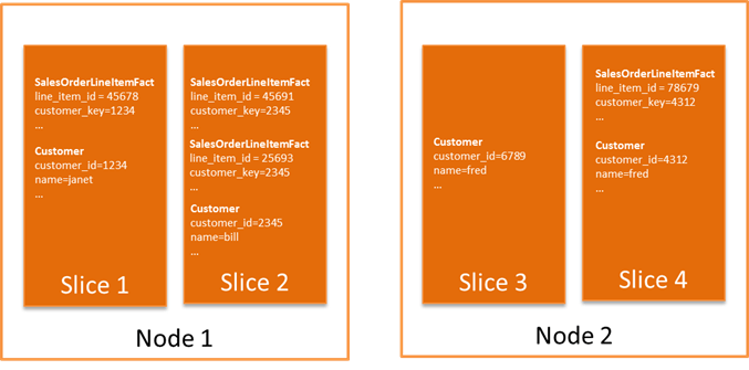
When you choose distribution keys, you should optimize for your most common joins while striving to spread data relatively evenly across the cluster for your tables. In the preceding example, if you were doing an operation on sales order, then Slice 2 needs to process two sales order lines while Slice 3, representing a customer with no orders, will do no work.

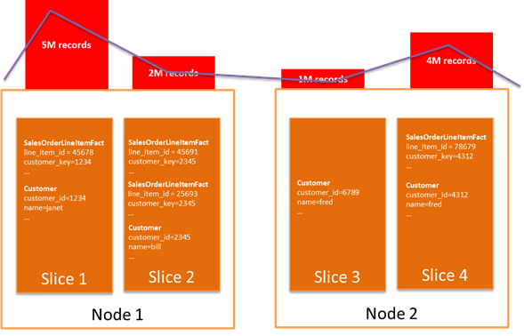
Figure 3 further illustrates how choosing a poor distribution key that excessively skews (unevenly distributes) data can degrade performance. In this scenario, when several large customers purchase a large proportion of the products from your company, distributing the fact table by customer_key results in a skew. The blue line represents compute utilization on each node.

In many cases, you may need to experiment with your data to see if the resulting distribution is reasonable. Sometimes a distribution key based upon the size of the joined tables seems like a good choice, but it ends up being a poor choice when you take skew into account. A common case is when two larger tables are joined on a particular column but the value in one of the tables is often null. For example, say you choose user_id for a distribution key in a table of web log file entries and a table of user profiles that are often joined, where the user_id in the log table is null if the user is not logged in. On the surface, user_id seems like a good choice, because both tables are large. However, the log table ends up with a large number of rows concentrated on the null column value, resulting in severe skew on one slice. For examples that show how to determine if your data is evenly distributed, see Distribution examples.

Amazon Redshift also has a distribution style of ALL. This distribution style replicates the table data once per node. Because the copy is used by all slices on the node, this distribution style has an impact on available storage. This distribution style is suitable for dimension tables that fit the following criteria:

• Reasonably large in size – You should experiment and measure the impact of this distribution style. Redshift moves data between nodes efficiently, so very small tables will not see significant gains.
• Slowly changing dimension data – Loading data into tables with a distribution style of ALL is expensive, but it can be worth it if the data is updated infrequently. Frequently changing dimension data with a distribution style of ALL increases load times significantly.
• Frequently joined on a column that is not a common distribution key – Typically this occurs because there is a larger dimension table joined with the fact table that uses a different distribution key or because the join key causes uneven data distribution when chosen as the distribution key.

Typically a star schema has a large fact table and numerous, comparatively smaller dimension tables. You can follow these steps to optimize the distribution choices for optimized table joins:

1. Identify large dimension tables used in joins.
2. Choose the large dimension that is most frequently joined as indicated by your query patterns.
3. Follow the guidelines in the preceding section to make sure that the foreign key to the dimension in the fact table gives relatively even distribution across your facts and that the primary/surrogate key for the dimension table is also relatively evenly distributed. If distribution is not relatively even, choose a different dimension.
4. Use the foreign key to the identified dimension as your fact table distribution key, and use the primary key in the dimension table as your dimension table distribution key.
5. Identify dimension tables that are suitable for a distribution style of ALL as described earlier in this article.
6. For the remainder of your dimension tables, define the primary key as the distribution key. The primary key does not typically exhibit significant data skew. If it does, then don’t define a distribution key.
7. Test your common queries and use the EXPLAIN command for any queries that need further tuning. For information about the EXPLAIN command, see the EXPLAIN command documentation.

Amazon Redshift is intelligent about minimizing the internode transmission of data to satisfy a query when it does joins, both by ordering how it executes elements of the join and by using techniques like hashing to minimize internode data transfer. Examples and techniques for performing joins are explained in EXPLAIN operators, Join examples, and the EXPLAIN command documentation. For more information about choosing a distribution key, see Choosing a data distribution style in the Amazon Redshift Database Developer Guide.

Sort Keys

You can improve query performance on Amazon Redshift by defining a sort key for each of your tables. A sort key determines how data is stored on disk for your table. The primary way a sort key improves query performance is by optimizing I/O operations when columns defined in the sort key are used in the where clause as a filtering condition (often called a filter predicate) or in operations like group by or order by. You should identify the most frequently used column for filtering and ordering operations in your dimension and fact tables as the sort key for each table.

If more than one column is typically used as a filter predicate, you can improve filtering efficiency by specifying multiple columns as part of the sort key. For example, let’s say the color and size columns are both specified in the sort key. If you filter on color = ‘red’ and size = ‘xl’, the use of color and size in the filtering and sort key makes the query execution more efficient. If you filter on color = ‘red’, the sort key will still be used to make the query more efficient since color is part of the leading key (the combination of the leading sort key columns). On the other hand, if you filter only for size=’xl’, then the sort key will not be used in the query execution because size is not part of the leading key. If the leading key is relatively unique (often called high cardinality), adding additional columns to your sort key will have little impact on query performance but will have a potential maintenance cost.

The sort key can have limited positive impact in other areas such as influencing more efficient joins and aggregations; however, the impact is not as reliable as the distribution key. For more information about defining sort keys, see Choosing sort keys in the Amazon Redshift Database Developer Guide.

Data Compression

Amazon Redshift optimizes the amount and speed of data I/O by using compression and purpose-built hardware. By default, Amazon Redshift analyzes the first 100,000 rows of data to determine the compression settings for each column when you copy data into an empty table. You can usually rely upon the Amazon Redshift logic to automatically choose the optimal compression type for you, but you can also choose to override these settings. Leaving compression turned on helps your queries to perform faster and minimizes the amount of physical storage your data consumes, thus allowing you to store larger datasets in your cluster. We strongly recommend that you use automatic compression. For more information about controlling compression options, see Choosing a column compression type.

This article will be a two-parter. I’m going to explore the pros and cons of the most popular programming languages with Lambda and the second one will contain benchmarks of said languages on Lambda. Hopefully, this will end up shedding some light on this particular subject.

So without further ado, here we go, with great biased and no benchmark to back my claims off(but do check back the blog soon and we’ll have those benchmarks ready for you).

If you are interested to learn AWS You can enroll for free live demo AWS Online Course

Java
Java has been in service for decades and is, to this day, a reliable option when choosing the backbone of your stack. With AWS Lambda is no different as it makes a strong candidate for your functions.

Java applications in AWS Lambda have the following merits.
Reliable and well-tested libraries. The libraries will make life easy for you through enhanced testability(test-ability?) and maintainability of AWS lambda tasks.

Predictive performance. While Java has slower spin up time, you can easily predict the memory needs of your functions and to counteract those dreaded colds starts you can just up your memory allocation.

Tooling Support. Java has a wide range of tooling support which includes Eclipse, IntelliJ IDEA, Maven, and Gradle among others.

If you’re wondering how Java remains an efficient AWS lambda language, here is the answer. Java has unique characteristics like multi-thread concurrency, platform independence, secure, and object-oriented.

Node.js
I’m definitely biased but Node.js is probably the best one in this list. I know it has it’s minuses but the overwhelming support that node had in the past years has to have its merits.

Why Node.js?
Modules. As of now, there are 1735 plugins on npm tagged “aws-lambda” which help developers with their applications in a lot of different ways from running Lambda locally to keeping vital functions warm to avoid clod-starts.

Spinup times. Node.js has better spin-up times than C# or Java which make it a better option for client facing applications that risk suffering from uneven traffic distribution.

Community. I’d be remiss if I wasn’t mentioning this as one of the major draw-ins of node is its community support on which you can always rely to find a solution to your problem.

Python
Python applications are everywhere. From GUI based desktops, web frameworks, operating systems, and enterprise applications. In the past few years, we’ve seen a lot of developers adopting python and it seems like this trend is not stopping.

Take your career to new heights of success with an Python Online course

The benefits of Python in AWS Lambda environments.
Unbelievable spin up times. Python is without a doubt the absolute winner when it comes to spinning up containers. It’s about 100 times faster than Java or C#.

Third party modules. Like npm, python has a wide variety of modules available. The feature helps ease interaction with other languages and platforms.

Easy to learn and community support If you are a beginner, programming languages can scare you. However, Python has extensive readability and a supportive community to help in its application. The Pythonistas have uploaded more than 145,000 support packages to help users.

Simplicity. With python you can void the overcomplicated arhitecture

Go
Introduction of GO language was a significant move forward for AWS Lambda. Although Go has its share of problems, it’s suitable for a serverless environment and the merits of Go are not to be ignored.

So, what is so outstanding about Go?
Go has a remarkable tenacity of 1.x. Unlike other languages like Java, C++, and others, Go has the highest tenacity. Such tenacity rate is a promise of a correct compilation of programs without constant alterations.

Go uses statistic binaries. It implies that the need for statistic linking is no more. Besides programming, AWS Lambda programs with Go would help enjoy forward compatibility.

Go offers stability It’s unique tooling, language design, and ecosystem makes the programming language shine.

Goroutines. Goroutines are a way of writing code which can run concurrently, whilst letting Go handle how many threads should actually be running at once which work amazingly in AWS Lambda.

Net.Core Language

Net.Core language popularity in programming stands out and it’s a welcomed addition to people already relying on AWS for running their .net applications.

NuGet Support. Just like all the other languages supported on Lambda, Net.core gets module support via NuGet which makes life for developers a lot easier.

Consistent performance. Net.Core has a more consistent performance result than Node.js or Python as a result of it’s less dynamic nature.

Faster execution Compared to Go, Net.Core has a faster execution time which is not something to be ignored.

6. Ruby
   If you’re an AWS customer, then Ruby is familiar to you. Ruby programming language stands out as it reduces complexities for AWS lambda users.

So, what are the benefits of Ruby in AWS lambda?
Third party module support. The language has unique modules that allow the addition of new elements of class hierarchy at runtime. Strong and supportive community. It thus makes it simple to use.

Clean Code. It’s clean code improves AWS Lambda performance.

Ruby is a relatively new addition to the AWS Lambda roaster but there is a lot of interest around it already. I look forward to seeing how far we can push Ruby using AWS Lambda.

Conclusion:

At first glance performance in a controlled, similar environment, running the same kind of functions isn’t all that different and until you get these to production you won’t be able to get a definitive conclusion. Stay tuned for the follow up for this article which will contain an updated benchmark of all the Languages supported by AWS Lambda in 2019.

Amazon CloudFront is a web service that speeds up distribution of your static and dynamic web content, such as .html, .css, .js, and image files, to your users. CloudFront delivers your content through a worldwide network of data centers called edge locations. When a user requests content that you’re serving with CloudFront, the user is routed to the edge location that provides the lowest latency (time delay), so that content is delivered with the best possible performance.

To get in depth knowledge on AWS you can enroll for free live demo AWS Online Course

If the content is already in the edge location with the lowest latency, CloudFront delivers it immediately.

If the content is not in that edge location, CloudFront retrieves it from an origin that you’ve defined—such as an Amazon S3 bucket, a MediaPackage channel, or an HTTP server (for example, a web server) that you have identified as the source for the definitive version of your content.

As an example, suppose that you’re serving an image from a traditional web server, not from CloudFront. For example, you might serve an image, sunsetphoto.png, using the URL http://example.com/sunsetphoto.png.

Your users can easily navigate to this URL and see the image. But they probably don’t know that their request was routed from one network to another—through the complex collection of interconnected networks that comprise the internet—until the image was found.

CloudFront speeds up the distribution of your content by routing each user request through the AWS backbone network to the edge location that can best serve your content. Typically, this is a CloudFront edge server that provides the fastest delivery to the viewer. Using the AWS network dramatically reduces the number of networks that your users’ requests must pass through, which improves performance. Users get lower latency—the time it takes to load the first byte of the file—and higher data transfer rates.

You also get increased reliability and availability because copies of your files (also known as objects) are now held (or cached) in multiple edge locations around the world.

How You Set Up Cloud Front to Deliver Content

You create a CloudFront distribution to tell CloudFront where you want content to be delivered from, and the details about how to track and manage content delivery. Then CloudFront uses computers—edge servers—that are close to your viewers to deliver that content quickly when someone wants to see it or use it.

How You Configure CloudFront to Deliver Your Content

1. You specify origin servers, like an Amazon S3 bucket or your own HTTP server, from which CloudFront gets your files which will then be distributed from CloudFront edge locations all over the world.An origin server stores the original, definitive version of your objects. If you’re serving content over HTTP, your origin server is either an Amazon S3 bucket or an HTTP server, such as a web server. Your HTTP server can run on an Amazon Elastic Compute Cloud (Amazon EC2) instance or on a server that you manage; these servers are also known as custom origins.If you use the Adobe Media Server RTMP protocol to distribute media files on demand, your origin server is always an Amazon S3 bucket.
2. You upload your files to your origin servers. Your files, also known as objects, typically include web pages, images, and media files, but can be anything that can be served over HTTP or a supported version of Adobe RTMP, the protocol used by Adobe Flash Media Server.If you’re using an Amazon S3 bucket as an origin server, you can make the objects in your bucket publicly readable, so that anyone who knows the CloudFront URLs for your objects can access them. You also have the option of keeping objects private and controlling who accesses them.
3. You create a CloudFront distribution, which tells CloudFront which origin servers to get your files from when users request the files through your web site or application. At the same time, you specify details such as whether you want CloudFront to log all requests and whether you want the distribution to be enabled as soon as it’s created.
4. CloudFront assigns a domain name to your new distribution that you can see in the CloudFront console, or that is returned in the response to a programmatic request, for example, an API request. If you like, you can add an alternate domain name to use instead.
5. CloudFront sends your distribution’s configuration (but not your content) to all of its edge locations or points of presence (POPs)— collections of servers in geographically-dispersed data centers where CloudFront caches copies of your files.

Or you can set up CloudFront to use your own domain name with your distribution. In that case, the URL might be http://www.example.com/logo.jpg.

Optionally, you can configure your origin server to add headers to the files, to indicate how long you want the files to stay in the cache in CloudFront edge locations. By default, each file stays in an edge location for 24 hours before it expires. The minimum expiration time is 0 seconds; there isn’t a maximum expiration time limit.

The AWS Console mobile app, provided by Amazon Web Services, allows its users to view resources for select services and also supports a limited set of management functions for select resource types.

Following are the various services and supported functions that can be accessed using the mobile app.

to get in depth knowledge on AWS you can enroll for free live demo AWS Online Training

EC2 (Elastic Compute Cloud)

• Browse, filter and search instances.
• View configuration details.
• Check status of CloudWatch metrics and alarms.
• Perform operations over instances like start, stop, reboot, termination.
• Manage security group rules.
• Manage Elastic IP Addresses.
• View block devices.

Elastic Load Balancing

• Browse, filter and search load balancers.
• View configuration details of attached instances.
• Add and remove instances from load balancers.

S3

• Browse buckets and view their properties.
• View properties of objects.

Route 53

• Browse and view hosted zones.
• Browse and view details of record sets.

RDS (Relational Database Service)

• Browse, filter, search and reboot instances.
• View configuration details, security and network settings.

Auto Scaling

• View group details, policies, metrics and alarms.
• Manage the number of instances as per the situation.

Elastic Beanstalk

• View applications and events.
• View environment configuration and swap environment CNAMEs.
• Restart app servers.

DynamoDB

• View tables and their details like metrics, index, alarms, etc.

CloudFormation

• View stack status, tags, parameters, output, events, and resources.

OpsWorks

• View configuration details of stack, layers, instances and applications.
• View instances, its logs, and reboot them.

CloudWatch

• View CloudWatch graphs of resources.
• List CloudWatch alarms by status and time.
• Action configurations for alarms.

Services Dashboard

• Provides information of available services and their status.
• All information related to the billing of the user.
• Switch the users to see the resources in multiple accounts.

Features of AWS Mobile App

To have access to the AWS Mobile App, we must have an existing AWS account. Simply create an identity using the account credentials and select the region in the menu. This app allows us to stay signed in to multiple identities at the same time.

For security reasons, it is recommended to secure the device with a passcode and to use an IAM user’s credentials to log in to the app. In case the device is lost, then the IAM user can be deactivated to prevent unauthorized access.

Root accounts cannot be deactivated via mobile console. While using AWS Multi-Factor Authentication (MFA), it is recommended to use either a hardware MFA device or a virtual MFA on a separate mobile device for account security reasons.